Unit 4 Video Notes

Video 1

This video went over two aspects of money. It first talked about the types of money listed as commodity, representative, and fiat money. Commodity money is a thing that has an independent function without being used as money while representative money is something that represents a valuable metal. Fiat money is money backed by the government. Functions of money include being a medium of exchange, store of value and unit of account.  The first two functions mean to use money to purchase something and save it for later. The unit of account means that the price of a product implies its worth.

Video 2

• The money demand slope is negative since the relationship between interest rates and quantity of money are inversely related. 
• The money supply line is vertical because it is not affected by the interest rate. It can only change by the Fed. 
• In order to control interest rates, the money supply has to be manipulated. 
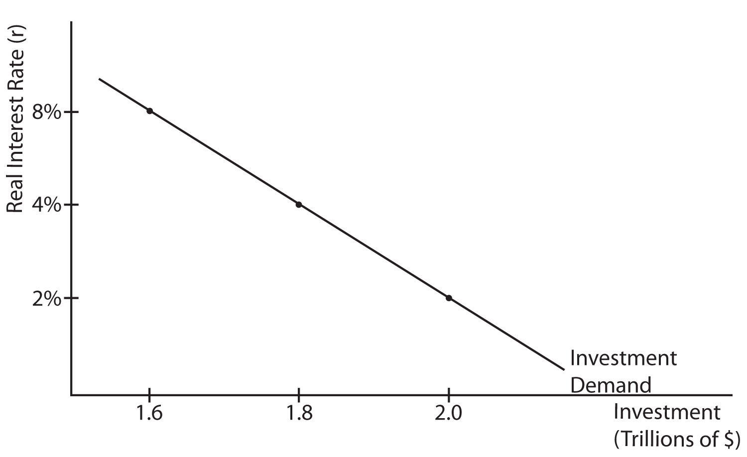
• Instability in interest rates leads to instability in investment and spending which leads to uncertainty in changes in aggregate demand.

Video 3

• Reserve ratio is a tool of the Fed in monetary policy. 
• Lowering it is seen in expansionary policy while raising the ratio is seen in contractionary policy. 
• It is less used compared to other tools. 
• The Discount Rate is another tool which is the interest rate the Fed charges to banks when the Fed lends out money. 
• It works similarly to reserve ratio in how the Fed uses it. 
• It does have a low impact. 
• Bonds and Securities are another tool of monetary policy. 
• Buying them is a part of expansionary policy while selling them is a part of contractionary policy. 
• These actions fall under open market operations.
• Federal funds rate works between fellow banks and not the Fed. It is the rate at which they borrow from each other.

Video 4

• Loanable funds is the amount of available money that people can borrow. 
• The demand for loanable funds is downward sloping just like the money demand slope. The supply of loanable funds is based on savings. 
• The supply shifts based on peoples' incentive to save. 
• Government deficit spending is shown by an increase in demand of loanable funds. To show an increase in interest rates, a decrease happens in the supply of loanable funds.

Video 5

• The money creation process explains the spending in an economy. 
• Money is created by making loans. 
• The loan amount multiplied by the money multiplier shows how much money is created. 
• In order to use the formula to find the amount of money created, the reserve requirement needs to be known. 
• The process works assuming that banks hold no excess reserves. Otherwise, the final amount will decrease.

Video 6

• Deficit spending affects the money market, the loanable funds market, and the aggregate demand and supply curve. 
• The demand for money increases. 
• The demand for loanable funds increases or the supply of loanable funds decreases.
• Aggregate demand will increase.
• A change in the supply of money influences the price level.
• Fisher Effect - Interest rates and inflation change at the same rate. 

Fiscal Policy

Fiscal Policy

• The change in expenditures or tax revenue of the federal government
• Can either increase or decrease taxes or spending

Types of Budget

• Balanced Budget = Rev. = Expenditures
• Deficit = Rev. < Expenditures
• When in deficit, gov. borrows from
• Individuals
• Corporations
• Financial institutions
• Foreign entities and countires
• Surplus = Rev. > Expenditures
• Gov. Debt = Sum of deficits - sum of surplus
• Discretionary (action) -
• Expansionary when in deficit
• Combats recession
• Increased spendng; Decreased taxes
• Contractionary when in surplus
• Combats inflation
• Decreased spending; Increased taxes
• Increase/decrease gov. spending or taxes to get back FE (Fiscal policy response to economic problems)
• Non-discretionary (wait)
• Automatic or built-in stabilizers - include unemployment compensation and marginal taxes;  they happen without policy makers

Tax Systems

• Progressive - Avg. tax rate rises with GDP (Tax revenue/GDP)
• Proportional - Avg. tax rate remains constant as GDP changes
• Regressive - Avg. tax rate falls with GDP
• More progressive = more stability

Consumption and Saving and Multipliers

Disposable Income

• The income after taxes [Gross - Taxes]
• Consume or save (Spend or not spend)
• Consumption - Restricted by DI & propensity to save
• If DI = 0, autonomous consumption and dissaving

• Saving - Restricted by DI & propensity to consume
• If DI = 0, no saving

• APC/APS = Average propensity to consume/save
• APC + APC = 1
• 1 - APC = APS
• 1 - APS = APC
• -APS or when APC > 1 -> Dissaving

Multipliers

• MPC + MPS = 1
• MPC = 1- MPS
• MPS = 1 - MPC
• MPC
• Marginal ... Fraction of any change in DI consumed 
• (Change in Consumption/Change in DI)
• MPS
• Fraction of DI saved
• (Change in Saving/Change in DI)
• Spending Multiplier Effect
• Initial change in spending; causes larger change in AS or AD
• (1/(1-MPC)) or 1/MPS
• Multiplier = (Change in AD/Change in C, Ig, G, or Xn)
• Positive is increase; Negative is decrease
• Tax Multiplier
• Reverse multiplier because it leaves circular flow
• Tax cut is positive because money enters circular flow
• Always negative
• -(MPC/(1-MPC)) or -(MPC/MPS)
• Multiplier = (Change in AD/Change in C, Ig, G, or Xn)

Classical vs. Keynesian

Classical 

• Followers
• Adam Smith
• J.B. Say
• David Ricard
• Alfred Marshall
• Say's Law
• Supply creates own demand
• Production = Income = Spending
• Underspending unlikely
• Whatever output produced will be demanded
• Savings and investment
• Savings = Investment income
• Savings (Leakage) = Investment (Injection)
• Loanable Funds Market

• Wage/Price Flexibility
• Downward
• Supply Curve
• Vertical
• Output and Employment
• Determined by AS
• Unemployment
• Rarely exists because of wage/price flexibility
• Cause: external (war)
• Aggregate Demand
• Determines PL
• Stable if money supply is stable
• Basic equation
• MV = PQ
• 1965 - 1972
• Role of government
• Monetary policy maintains steady money supply
• Laissez-faire is best
• Self regulating economy
• Inflation
• Too much money
• How long the short run is
• Short time
• Emphasis today
• Microeconomics
• Other
• Competition is good
• Invisible Hand
• Long run - Balance @ FE
• Trickle-Down effect - Help rich 1st, everyone else 2nd

Keynesian

• Followers
• J.B. Keynes
• Say's Law
• Depressions refute Say's Law
• Demand creates own supply
• Underspending persists
• Savings and investments
• Savings not equal to investment
• Different motivations
• Savings
• Future needs
• Precaution
• Habit
• Income level
• Interest rate
• Investment
• Interest rate
• Rate of profit
• Expectations
• Loanable Funds Market
• Investment from savings, cash, checking accounts
• Lending creates money -> Supply of money increases
• Inflation and unemployment are unstable
• Wage/price inflexibility
• Prices and wages inflexible downward
• Ratchet effect
• Supply curve
• Horizontal
• Output and Employment
• Determined by AD
• Unemployment
• Usually exists
• Causes:
• External (war)
• Internal (Savings not equal to investment
• Aggregate Demand
• Changes due to determinants
• Unstable even if money supply is stable due to fluctuations in investment spending
• Basic equation
• C + Ig + G + Xn 
• 1973 - Present
• Role of Government
• Fiscal Policy - Tax and spend
• Active government
• Economy is not self regulating
• Inflation 
• Too much demand
• How long the short run is
• Long time
• Emphasis Today
• Macroeconomics
• Other
• Flawed competition
• AD is key; not AS
• Leaks + Savings = Recession
• Ratchet effects and Sticky Wages block Say's Law
• We are doomed in the long run

Investment Demand

• Investment - $ spent/expenditures on new plants/factories, capital equipment, technology, new homes, inventory.

Expected Rates of Return

• Invest based on cost/benefit analysis
• Benefits from expected rate of return
• Cost from interest costs
• Amount of investment from comparison of expected rate of return to interest cost
• Exp return > Interest Cost = Yes
• Exp return < Interest Cost = No
• r% vs. i%
• Nominal = observable rate of interest; Real takes out inflation, known ex post facto
• r% = i% - pi% -> bases investment decision

The Curve

• Downward sloping because high rates = less investment, vice versa
• Shifts 
• Cost of production 
• Low = right
• High = left
• Business Taxes
• Low = right
• High = left
• Tech Change
• New = right
• Lacking = Left
• Stock of Capital
• Low = right
• High = Left
• Expextations
• Positive = right
• Negative = left

Aggregate Supply

Aggregate Supply

• The level of real GDP that firms produce at each price level
• Long Run - Period where input $ are flexible & adjust to change in PL
• Real GDP is independent to PL
• Short Run - Input prices are rigid; they do not adjust 
• Real GDP related to PL
• LRAS - Shows full employment (analogous to PPC)
• Vertical @ full employent

Changes in SRAS

• An increase is represented as a shift to the right
• A decrease is represented as a shift to the left.
• Changes are based on cost of production per unit (Total input cost/total output)
• Determinants:
• Input Prices
• Domestic resources $ [75% on wages, Capital cost, Raw material]
• Foreign resource $
• Market Power ... Increase shifts left; Decrease shifts right
• Productivity - (Total output/total input)
• More productivity -> Low unit prod. $ -> SRAS shifts right
• Less productivity -> High unit prod. $ -> SRAS shifts left
• Legal Institution Environment
• Taxes & Subsidies 
• Taxes shift SRAS left
• Subsidies shift SRAS right
• Gov. regulation
• Regulation causes cost of compliance = SRAS <-
• Deregulation reduces compliance costs = SRAS->
• FE equilibrium occurs when AD crosses SRAS & LRAS @ same point

• Recessionary Gap - Occurs when equilibrium is below FE output
• Inflationary Gap - Equilibrium is above FE output
• SRAS 

• Nominal Wages - Amount of $ received by worker per unit of time
• Real Wages - Amount of goods/services worker can buy with nominal wages
• Sticky Wages - Set nominal wages from initial price levels
• Does not vary because labor contracts etc.

Aggregate Demand

Aggregate Demand

• Aggregate Demand - Demand by consumers, businesses, government, and foreign countires
• Change in price = Move along curve
• AD = C + I + G + Xn
• The curve is a downward slope because:
1. Real Balance Effect: Higher price -> Less purchase power of $
1. Reduced quantity of expenditures
2. Lower price levels -> Higher purchase power and expenditures
2. Interest Rate Effect: Higher price level -> Higher interest rates -> Less spending & investment
3. Foreign Trade Effect: US price level increase -> Foreign buyers buy less U.S and Americans buy foreign.

Determinants of AD

• Shifters = Expenditure approach of GDP
• Includes
• Change in C, I, Ig, Xn
• Multiplier that produces greater change than original in 4 comp.
• AD up = Right  :  AD down = Left
• Consumption: Affected by-
• Consumer Wealth - Right if more; Left if less
• Consumer Expectations - Positive goes right; Negative goes left
• Household Indebtedness - Right if less; Left if more
• Taxes - Right if less; Left if more
• Gross Private Investment: Affected by:
• Real Interest Rate - Right if lower; Left if higher
• Expected Returns - Right if higher; Left if lower
• Influenced by: 
• Profit Expectations 
• Technology
• Degree of excess capacity
• Business taxes
• Government Spending:
• More leads to right
• Less leads to left
• Net Exports: Affected by - 
• Relative Income
• Strong foreign economy -> More exports -> Right
• Weak foreign economy -> Less exports -> Left
• Exchange rates
• Strong $ -> More imports; Fewer exports -> Left
• Weak $ -> Less imports; More exports -> Right